


 Call Us



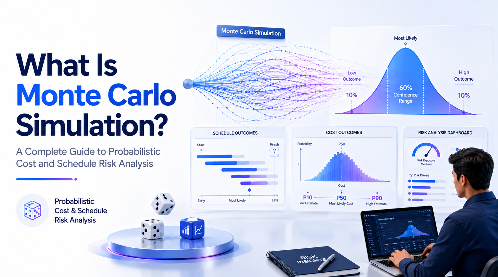
Monte Carlo simulation is a quantitative risk analysis technique that runs a project's cost or schedule model thousands of times, each time drawing random values from three-point (optimistic, most likely, pessimistic) estimates for every activity, to produce a full probability distribution of possible outcomes instead of one number. The output is usually read as an S-curve, from which planners pick a confidence level, commonly P50, P80 or P90, to set a realistic budget or finish date and to size the contingency reserve above the deterministic estimate. It sits inside the quantitative risk analysis techniques tested on the PMI Scheduling Professional (PMI-SP) exam and is a named technique in PMI's Risk Management Professional exam content outline. This guide walks through the mechanics, a full worked example, and how the analysis is actually run.
Key Highlights
- Monte Carlo simulation converts three-point (optimistic, most likely, pessimistic) estimates into thousands of randomly sampled iterations, producing a probability distribution rather than a single deterministic number.
- The output is displayed as an S-curve (cumulative distribution function), from which P50, P80 and P90 confidence levels are read directly.
- Contingency reserve is calculated as the gap between the chosen confidence level (typically P80) and the deterministic base estimate, giving a defensible, data-backed reserve figure instead of a flat percentage.
- It is explicitly named as a quantitative risk analysis technique in PMI's examination content outlines and is most directly relevant to the PMI-RMP and PMI-SP credentials, and to the quantitative risk chapter within PMP preparation.
- Correlation between activities and risks is the single most common modelling failure; treating dependent risks as independent understates the true probability of overrun.
- AI-assisted platforms are increasingly auto-fitting input distributions from historical project data and flagging which risks drive the tail of the output distribution, but they do not replace the judgement calls behind the model.
- Enterprise adoption clusters in infrastructure, defence, construction, and large IT programmes, where cost and schedule overrun exposure is high enough to justify the modelling effort.
What Is Monte Carlo Simulation and Who Governs It
Monte Carlo simulation is a computational technique that models uncertainty by repeatedly sampling from probability distributions assigned to uncertain inputs (activity durations, unit costs, risk event probabilities and impacts) and recalculating the project outcome for every sample. Run often enough, typically several thousand iterations, the collected results form a probability distribution of total project cost or duration rather than a single figure. It is one of several quantitative risk analysis techniques, alongside sensitivity analysis, decision tree analysis and expected monetary value (EMV) calculations, that are used once qualitative risk analysis has narrowed the risk register down to the risks worth modelling numerically.
There is no separate certifying body for Monte Carlo simulation itself; it is governed by the standards and exam content outlines of the Project Management Institute (PMI). PMI's Risk Management Professional (PMI-RMP) Examination Content Outline explicitly lists Monte Carlo simulation among the numerical techniques candidates must be able to apply and interpret, alongside sensitivity analysis and decision trees, and places quantitative analysis as one of the exam's most heavily weighted domains, as set out in PMI's updated 2024 RMP Examination Content Outline. The technique is also referenced within the schedule risk analysis content of the PMI-SP certification, and within the broader risk management knowledge covered in PMP certification training, since Monte Carlo output is the natural next step after building a risk register and estimating individual activities.
1. Three-Point Estimates as the Raw Input
Every uncertain activity, cost line or risk event is expressed as a range rather than a single figure: an optimistic value (O), a most likely value (M), and a pessimistic value (P). This is the same three-point structure used in PERT three-point estimating, and it is usually shaped into a triangular or Beta-PERT probability distribution before it is fed into the simulation engine. A deterministic plan, by contrast, uses only the most-likely value, which is precisely what a Monte Carlo model is built to correct for. Related estimating approaches, including analogous, parametric and bottom-up estimating, feed the same three-point structure before it reaches the simulation stage.
2. Iterations: Sampling the Model Thousands of Times
The simulation engine draws one random value from each input distribution, calculates the resulting total (summing activity durations along the critical path, or line-item costs), and records that single outcome. This is repeated, commonly 5,000 to 10,000 times for a project-level model, so that rare combinations of pessimistic values across multiple activities are captured, not just the average case. Too few iterations leave the tail of the distribution unstable; the percentile values will shift noticeably if the run is repeated.
3. The Output: An S-Curve, Not a Single Number
Plotting all recorded outcomes as a cumulative distribution produces the characteristic S-shaped curve: the x-axis is cost or duration, the y-axis is the cumulative probability of finishing at or below that value. A steep S-curve indicates concentrated, lower-uncertainty outcomes; a flat, stretched-out curve signals wide uncertainty that a single-point estimate would have hidden entirely.
4. Reading Confidence Levels: P50, P80 and P90
Percentiles are read straight off the S-curve. P50 is the median outcome, an even chance of finishing above or below it. P80 means 80% of the simulated iterations finished at or below that value, leaving a 20% chance of overrun. P90 is more conservative again, leaving only a 10% chance of overrun. Most organisations commit to P80 for a working budget or schedule baseline and reserve P90 for board-level or contractually binding commitments, though the right choice depends on the organisation's risk appetite rather than a fixed rule.
| Confidence Level | Meaning | Typical Use |
| P50 | 50% probability of finishing at or below this cost/date | Internal planning baseline; not a safe committed figure on its own |
| P80 | 80% probability of finishing at or below this cost/date | Most common basis for setting contingency reserve and working budget |
| P90 | 90% probability of finishing at or below this cost/date | Conservative commitments, fixed-price contracts, board-approved reserves |
Worked Example: From Three-Point Estimates to a Contingency Figure
The following example is illustrative and built specifically for this guide, not a real project. A mid-size ERP rollout has three sequential phases on its critical path, each estimated with optimistic (O), most likely (M) and pessimistic (P) durations in weeks:
| Phase | Optimistic (O) | Most Likely (M) | Pessimistic (P) | PERT Expected, (O+4M+P)/6 |
| Design | 8 | 10 | 16 | 10.67 |
| Build | 14 | 18 | 30 | 19.33 |
| Test and Cutover | 6 | 8 | 14 | 8.67 |
A traditional deterministic schedule simply sums the most-likely column: 10 + 18 + 8 = 36 weeks, treated as the committed plan. Feeding the same three ranges into a Monte Carlo engine as triangular distributions and running 10,000 iterations produces a full S-curve of possible total durations. In this illustrative run, the simulation returns a P50 of roughly 39 weeks, a P80 of roughly 43 weeks and a P90 of roughly 46 weeks. Converting duration to cost at an assumed burn rate of $50,000 per week, the deterministic plan implies a cost of $1.8 million, while the P80 duration implies roughly $2.15 million. The contingency reserve at P80 is therefore approximately $350,000, about 19% above the deterministic figure, a number the project team can defend to a sponsor because it is tied to a stated 80% confidence level rather than a flat, unexplained percentage added for comfort. This is the mechanic behind the reserve-analysis workflow described in Simpliaxis's guide to reserve analysis in project management.
How AI-Assisted Platforms Are Changing the Mechanics
The manual steps above, choosing a distribution shape, entering three points by hand, and re-running iterations after every schedule change, are increasingly assisted by software rather than eliminated. Three categories of behaviour are now common in current risk and scheduling platforms:
- Automated distribution fitting from historical project data, where the software statistically fits a probability distribution to a library of past activity durations or cost lines instead of asking a planner to guess optimistic and pessimistic bounds from scratch.
- AI-drafted plain-language exposure narratives, where the platform turns the raw S-curve and percentile table into a short written summary of what is driving the risk, aimed at a sponsor who will not read a probability distribution unassisted.
- Predictive flagging of tail-risk drivers, where the software ranks which specific risks or activities contribute most to the spread between P50 and P90, functioning as an automated, continuously updated version of a sensitivity or tornado chart.
What none of this replaces is human judgement on three specific points: whether the historical data being fitted is actually a fair analogue for this project's context and not a different risk profile entirely; how much contingency a sponsor will realistically approve once the number leaves the model and enters a budget conversation; and whether P80, as opposed to P50 or P90, is the right target given this project's contractual terms and the organisation's actual appetite for risk. Those remain analyst decisions, not outputs a tool can generate on its own.
Monte Carlo Simulation vs Traditional Single-Point/Deterministic Estimating
| Dimension | Deterministic (Single-Point) Estimating | Monte Carlo Simulation |
| Input format | One value per activity or cost line (usually "most likely") | A range per activity or cost line (optimistic, most likely, pessimistic) |
| Output | A single total cost or duration figure | A full probability distribution and S-curve of possible totals |
| Handles correlation between risks | No, sums are additive and independent by default | Yes, correlations between activities or risks can be explicitly modelled |
| Confidence statement possible | None; the figure carries no stated probability of being met | Yes, e.g. "80% probability of finishing at or below this date/cost" |
| Contingency basis | Often a flat, judgement-based percentage add-on | Data-derived gap between the chosen confidence level and the base estimate |
| Effort and tooling required | Low; a spreadsheet sum is sufficient | Moderate to high; needs simulation software and calibrated input ranges |
| Best suited to | Small, low-uncertainty, low-value work packages | Complex, high-value or contractually significant cost and schedule commitments |
The two approaches are not mutually exclusive. Most mature project controls functions build the deterministic estimate first, using techniques such as three-point and PERT estimating, and then layer a Monte Carlo simulation on top of it specifically to quantify how much reserve that deterministic figure is missing.
Monte Carlo Simulation Career and Business Value
Quantitative risk analysis is one of the more differentiating skills a project professional can add on top of a base PMP certification, because it moves a practitioner from reporting risks qualitatively to defending a specific budget or schedule number with data. It is the core skill tested by the PMI-RMP credential and forms a meaningful part of the PMI-SP scheduling credential's content, both of which signal to employers that a candidate can build and interpret a simulation model rather than only recite risk terminology. In sectors that routinely run cost or schedule risk analysis, infrastructure, defence, construction, aerospace and large-scale IT programmes, the ability to translate a P80 output into a contingency figure a sponsor will actually approve is a distinct value-add over general risk management knowledge. As AI-assisted platforms absorb more of the mechanical work of fitting distributions and running iterations, the professional value of this skill is shifting away from performing the calculation and toward the judgement layered on top of it: choosing realistic input ranges and correlations for a specific project's context, and deciding which confidence level and contingency figure a given organisation should actually commit to.
Monte Carlo Simulation Common Risks and Mistakes
- Input ranges that are too narrow, where estimators anchor on the most likely value and set optimistic and pessimistic bounds too close to it, which understates true uncertainty in the output distribution.
- Ignoring correlation between activities or risks, treating dependent items as statistically independent when, in reality, a delay driver such as a weather event or a shared supplier affects multiple activities at once.
- Running too few iterations, which leaves percentile values unstable, especially at the tail (P90 and above), so the same model produces meaningfully different results on repeated runs.
- Treating the model as a black box and reporting whatever number it produces without validating that the model structure actually reflects the real project logic and dependencies.
- Confusing P50 with a safe committed figure, when by definition it carries only an even chance of being met or missed.
- Building a highly precise-looking simulation on top of poor-quality risk register inputs, which is simply garbage-in, garbage-out dressed up with statistical credibility.
- Overlooking that even a P90 or P95 output does not capture true black-swan, low-probability, high-impact events that sit outside the modelled input ranges entirely.
Employer Recognition and Enterprise Adoption
Monte Carlo-based cost and schedule risk analysis is a named, expected deliverable on many large infrastructure, defence, and capital construction programmes, where commercial software packages have made the technique accessible well beyond specialist statisticians. Adoption clusters most heavily where cost or schedule overrun exposure is financially material: infrastructure megaprojects, defence contracting, large enterprise software implementations, and multi-year research and development programmes are the environments where organisations most consistently build quantitative risk analysis into their standard planning process rather than treating it as optional. Employers in these sectors recognise PMI-RMP and PMI-SP credentials specifically because they signal that a candidate can run and interpret this kind of model, not only describe risk qualitatively. Adoption remains uneven outside these sectors, constrained less by the technique itself than by the time, historical data and specialist expertise needed to build a defensible model, which is exactly the gap that AI-assisted distribution fitting and narrative generation are starting to narrow.
Practical Workplace Application
Illustrative scenario: A programme manager on a data centre construction project has a deterministic schedule showing completion in 52 weeks. The sponsor wants a committed date to put into a contract. Rather than quoting 52 weeks with no stated confidence, the risk analyst runs a Monte Carlo simulation using three-point estimates for each major work package, correlating weather-sensitive activities together rather than treating them as independent. The resulting S-curve shows P50 at 53 weeks and P80 at 58 weeks. The team commits contractually to the P80 date and carries the six-week gap as an explicit schedule reserve, giving the sponsor a defensible answer when asked why the committed date is later than the "most likely" schedule.
Illustrative scenario: A PMO analyst supporting a portfolio of IT implementation projects uses an AI-assisted risk platform that automatically fits input distributions from the organisation's own database of past project durations, rather than asking each project manager to guess optimistic and pessimistic bounds from memory. The platform also generates a short plain-language narrative flagging that two specific integration risks are driving most of the spread between P50 and P90 on the current model. The analyst still has to judge whether those historical projects are a fair comparison for this particular implementation's vendor and scope, and still has to negotiate with the sponsor over whether the resulting contingency request is one the business will actually fund, decisions the platform surfaces information for but does not make.
How to Get Started with Monte Carlo Simulation
- Build a solid risk register first, since a Monte Carlo model is only as good as the risks and estimates fed into it; Simpliaxis's guide to risk registers in project management is a reasonable starting point.
- Practise three-point and PERT estimating on real work packages before attempting a full simulation, so that optimistic, most likely and pessimistic values reflect genuine judgement rather than guesswork; PERT three-point estimating is the direct input format Monte Carlo models depend on.
- Learn to read an S-curve and explain P50 versus P80 versus P90 in plain language to a non-technical sponsor, since the analysis has limited value if its output cannot be explained and acted on.
- Pursue formal grounding through PMP certification training for the broader risk management context, then PMI-SP certification for schedule-risk-specific depth, or explore Simpliaxis's wider project management certification course catalogue to plan a risk-specialist career path such as PMI-RMP.
- Get hands-on with an actual simulation tool on a low-stakes internal model before applying the technique to a contractually significant estimate, so mistakes around correlation and iteration count are caught early.
Conclusion
Monte Carlo simulation earns its place in quantitative risk analysis because it replaces a single, unqualified number with a stated probability, turning "the project will cost $1.8 million" into "there is an 80% chance the project will cost $2.15 million or less," and turning contingency reserve from a guess into a defensible, data-derived figure. Reading an S-curve, choosing an appropriate confidence level, and defending the resulting reserve to a sponsor are core competencies for anyone pursuing PMI-RMP, PMI-SP, or the quantitative risk components of the PMP. As AI-assisted platforms take over more of the mechanical work of fitting distributions and running iterations, the professional value of this skill is likely to concentrate even further in the judgement calls that sit around the model rather than the calculation itself, which is precisely the part of the skill that is hardest to automate.








 Lowest-Price Challenge











 Personalized Path


.webp)


 USA
USA  Canada
 India
India UK
UK Australia
 Singapore


