


 Call Us




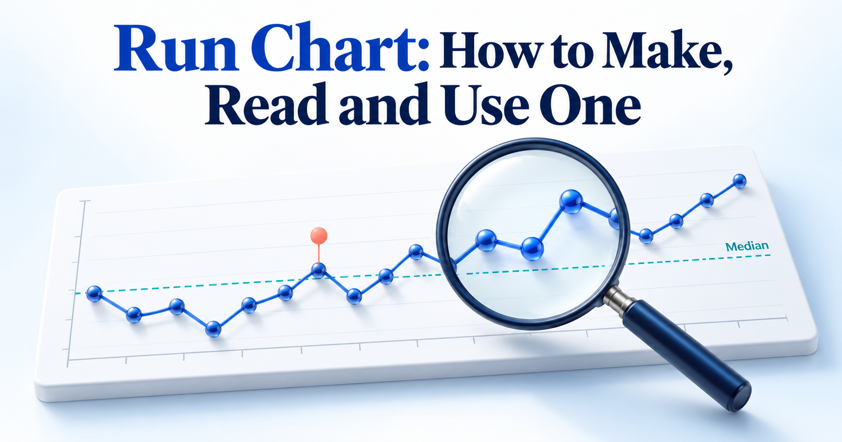
A run chart is a line chart of one process measure plotted in time order, with a horizontal line drawn at the median. When nothing in the process has changed, points should fall on either side of the median more or less at random, so the median gives you a fair yardstick for spotting real patterns. Four simple rules (shift, trend, number of runs and astronomical data points) help you judge whether a change is likely real or just normal ups and downs. That makes the run chart one of the quickest ways to check whether a quality improvement effort is actually working.
Introduction
Every process varies. Call handling time moves a little each day, defect counts rise and fall, and patients wait longer on some mornings than others. The hard part is telling the difference between normal ups and downs and a genuine change.
A single number rarely settles that question. Comparing last month's average with this month's can hide what happened in between, and one good week can look like a breakthrough when it is just chance. Teams then celebrate changes that did nothing or abandon ones that were working.
This is where a run chart helps. It is a simple data visualization tool that puts your measurements in time order and reads them against the median. Quality professionals, Six Sigma practitioners, project managers and healthcare teams use it because it needs very little statistics and gives a fair, visual answer to one practical question: is the process actually changing?
What Is a Run Chart?
A run chart is a graph that shows how one measurement changes over time. Values sit on the vertical axis, time or sequence runs along the horizontal axis, and a median line acts as the reference point. NIST calls the same graph a run-sequence plot and uses it to check for shifts in level, changes in spread and outliers (NIST e-Handbook: run-sequence plot). For general background, seeRun chart on Wikipedia.
The run chart is often taught alongside the seven QC tools, such as check sheets, histograms andPareto analysis. Those tools show how data is spread or which problems happen most. A run chart adds the time dimension, so teams use it to understand current performance, test whether a change led to improvement and check that gains are holding.
Parts of a Run Chart
- Horizontal (X) axis: time or sequence, such as days, weeks, batches or patient visits, in the order they occurred.
- Vertical (Y) axis: the measure being tracked, with its unit, for example minutes, defects per 1,000 units or percentage on time.
- Data points: one point per observation or per period.
- Connecting lines: lines that join the points in order. They add no new data but make the direction of movement easy to follow.
- Median line: a horizontal line at the median value, with half the points above and half below. The median is used instead of the mean because one extreme value cannot pull it up or down.
- Annotations: short notes marking when a change was introduced, or an unusual event occurred.
Run Chart Diagram Explained
The run chart diagram below shows 12 weeks ofthroughput for a software delivery team, measured as user stories completed per week. Values move between 12 and 18 and cross the median of 15 several times, while two weeks land exactly on the median.
There is no long streak on one side and no steady climb. This is what common cause variation, the normal background noise of a stable process, usually looks like. A throughput run chart like this makes a good baseline for a project management run chart before the team tests any change.

Read it from left to right: each dot is one week, and its position relative to the dashed median line is what the interpretation rules look at.
How to Make a Run Chart Step by Step
You can draw a run chart on paper, in a spreadsheet or in statistical software. The steps are the same either way.
Choose the Measure
Pick one measure that matters to your customer or your process, such as customer waiting time, production defects, delivery time, patient waiting time or weekly project throughput. Then define it precisely: what counts, the unit, and when it is recorded. "Resolution time" means little until you decide whether the clock starts when a ticket is logged or when it is assigned.
If you work in Six Sigma, your choice will usually connect to theSix Sigma metricsthe project is trying to move. Measures you can record weekly or daily are better than quarterly ones, because you collect enough points to learn from much sooner.
Collect Time-Ordered Data
Record every value with its date or sequence number. Order is the whole point of a run chart. If the data is sorted by size or mixed up, the patterns you are looking for disappear.
Keep the method consistent. The same definition, the same tool and the same way of counting should apply to every point. If you are unsure whether the measurement itself is reliable, check it with ameasurement system analysisbefore reading too much into the chart. IHI suggests having at least 10 data points before you calculate and draw the median.
Plot Points and the Median
Take the throughput data from the diagram above. The 12 weekly values, in time order, are:
14, 16, 13, 15, 17, 18, 15, 12, 13, 16, 14, 17
- Plot each value against its week and join the points with a line.
- Sort the values from lowest to highest: 12, 13, 13, 14, 14, 15, 15, 16, 16, 17, 17, 18.
- Find the middle. With an even number of values (12), average the 6th and 7th values: (15 + 15) / 2 = 15. With an odd number, the median is simply the middle value.
- Draw a horizontal line at 15 across the whole chart.
Repeated values stay in the sorted list; both 13s and both 15s count. Points that equal the median (weeks 4 and 7 here) sit on the line. You plot them normally but skip them when applying the shift and run rules, which leaves 10 "useful" observations in this example.
When you plan to test a change, calculate the median from the baseline period only and extend that line forward. New results are then judged against old performance rather than against a median they helped to create.
Annotate Changes
Mark the chart wherever something changed: a new procedure, a training session, a new tool, a staffing change. Keep each note short and dated, for example "Week 13: stand-up moved to 9:30 am".
Note outside events too, such as public holidays, system outages or a supplier problem. TheIHI: run chart tool recommends annotating both tests of change and external events. Without these notes, you may later spot a pattern but have no record of what might explain it.
Interpreting Run Charts
Interpreting run charts comes down to four rules, widely taught through IHI and the healthcare improvement literature. Three of them are probability based: each pattern has roughly a 5% chance or less of appearing when the process has not really changed. The fourth relies on judgement.
One rule is enough to signal a likely non-random change. You do not need all four. Keep in mind that these run chart rules work with the median line, not with control limits.
Shift Rule
A shift is six or more consecutive points all above or all below the median. It suggests the process has settled at a new level, which is usually the signal you hope to see after an improvement.
To count, start at the first point on one side and keep going while points stay on that side. A point that falls exactly on the median is skipped: it neither adds to the count nor breaks it. Say the median is 30 minutes and the next values are 28, 27, 30, 29, 26, 25 and 27. Skip the 30, and six points remain below the median, which makes a shift.
Some references suggest seven or eight points for longer data sets. Whichever convention your team uses, apply it consistently.
Trend Rule
A trend is five or more consecutive points all going up or all going down. It points to a gradual drift rather than a step change.
Repeated values do not count as an increase or a decrease. If two neighbouring points are equal, count only one of them and carry on. For example, daily defects of 9, 8, 8, 7, 5, 4 and 3 contain a repeated 8. Count it once and you get six points (9, 8, 7, 5, 4, 3) all falling, which is a trend. Two or three points moving the same way is not a trend, however tempting it looks.
Too Many or Too Few Runs
A run is one or more consecutive points on the same side of the median. Points on the median are ignored. A quick way to count runs is to count how many times the line crosses the median and add one.
In the throughput example, the 10 useful points form 8 runs: below, above, below, above (two weeks), below (two weeks), above, below, above. The expected range comes from a probability table based on the number of useful observations. A few rows are shown below.
Useful observations (not on median) | Too few if runs are below | Too many if runs are above |
10 | 3 | 9 |
15 | 5 | 12 |
20 | 6 | 16 |
25 | 8 | 18 |
30 | 11 | 21 |
With 10 useful observations, 3 - 9 runs are normal, so 8 runs give no signal. Too few runs means the data stays on one side for long stretches, which often comes with a shift. Too many runs means the line flips across the median more than chance allows, which can happen when data from two sources is mixed, such as day and night shifts. Always look up the limits for your own number of points rather than using a fixed figure.
Astronomical Data Points
An astronomical data point is a value so different from the rest that anyone looking at the chart would agree it is unusual. Every data set has a highest and a lowest value, and those are not automatically astronomical.
Imagine call waiting times sitting between 4 and 7 minutes for weeks, then one day reaching 19 minutes during a phone system outage. That point deserves investigation. Start by checking for a data entry error, then look for a specific event.
This rule is a visual judgement, not a statistical test. It helps to separate two kinds of variation. Common cause variation is the normal noise built into a process. Special cause variation comes from something specific and unusual. An astronomical point hints at a special cause, but one exceptional value is not proof that a process has improved or worsened.
Example of Run Chart
Each run chart example below uses realistic data to show how the rules work in practice.
Quality Improvement Run Chart Example
An IT service desk wants to reduce the time it takes to resolve support tickets. The measure is average resolution time per week, in hours, from ticket logged to ticket closed.
The baseline for weeks 1 to 10 is 31, 28, 33, 29, 30, 27, 32, 30, 29 and 31 hours. Sorted, that is 27, 28, 29, 29, 30, 30, 31, 31, 32, 33, so the median is (30 + 30) / 2 = 30 hours. The team freezes this median and extends it across the chart.
In week 11, the team introduces a triage step and a shared knowledge base, and marks the change on the chart. Weeks 11 - 20 come in at 28, 27, 29, 26, 25, 27, 24, 23, 25 and 24 hours.

Here is what the four rules show:
- Shift: all ten points from week 11 onwards sit below the 30-hour median, well past the six needed.
- Trend: the longest fall is three points in a row, so there is no trend.
- Runs: the 18 useful points form 8 runs, inside the expected range of 6 to 14.
- Astronomical point: none.
The process has moved to a lower level, and the median for weeks 11 to 20 is 25.5 hours. A run chart cannot prove the triage step alone caused this, but the timing matches the annotation. The team keeps plotting to confirm the gain holds before setting a new median. Notice that one rule produced the signal while the others stayed quiet.
Run Chart in Healthcare
Run charts are a staple of healthcare quality improvement, partly because they are easy to update weekly on a ward noticeboard. Here, an outpatient clinic wants to cut the time patients wait between check-in and consultation, measured as average weekly waiting time in minutes.
Baseline weeks 1 to 10 are 42, 38, 45, 40, 44, 39, 41, 47, 43 and 40 minutes, giving a median of (41 + 42) / 2 = 41.5 minutes. The team then runs two PDSA (Plan-Do-Study-Act) cycles and annotates each one:
- PDSA 1 (week 11): reminder calls asking patients to arrive with their documents ready. Weeks 11 to 14 come in at 40, 44, 39 and 42.
- PDSA 2 (week 15): staggered appointment slots in place of block booking. Weeks 15 to 20 come in at 37, 36, 34, 35, 32 and 31.
After PDSA 1, points keep crossing the median, so there is no signal. That is still useful learning: the team adapted its approach instead of assuming success. After PDSA 2, weeks 15 to 20 give six consecutive points below 41.5, which meets the shift rule. There is no trend, as the longest fall is four points, and the number of runs stays within the expected range.
The median for weeks 15 to 20 is 34.5 minutes. The clinic has reasonable evidence that staggered slots shortened waits and will keep measuring before making the change permanent.
Run Charts and Control Charts
A control chart is the run chart's more statistical relative. It also plots data in time order, but it uses a centre line (usually the mean) and adds upper and lower control limits calculated from the process's own variation (ASQ: control chart). Run charts and control charts answer the same basic question, whether the process is changing, with different levels of statistical depth. Many teams use both at different stages.
Comparison Table
Aspect | Run chart | Control chart |
| Purpose | Show performance over time and detect non-random change | Monitor stability and separate common cause from special cause variation |
| Centre line | Median | Usually the mean (average) |
| Control limits | None | Upper and lower limits calculated from the data |
| Statistical interpretation | Four rules: shift, trend, runs, astronomical point | Points beyond limits plus run and pattern rules |
| Complexity | Low; needs only a median | Moderate; needs the right chart type and formulas |
| Data requirements | Useful from about 10 points | Typically 20 or more points or subgroups for reliable limits |
| Common applications | Improvement projects, PDSA tests, team dashboards | Ongoing process monitoring, SPC, the Control phase of DMAIC |
| When to use | Early in a project or when testing changes | When you need to judge stability or hold a process steady |
The run chart vs control chart choice is not about which is better. A run chart is quicker to build and explain, while a control chart gives sharper evidence about the type of variation.
When to Upgrade to a Control Chart
Consider moving to a control chart when you need a firmer answer about whether variation is common cause or special cause, when you are about to assess process capability, or when a process has to be monitored for months rather than weeks. Having 20 or more data points also makes the limits more dependable. Simpliaxis covers the different types and how to read them in its guide tocontrol charts.
In Six Sigma projects, the switch often happens at the end of the Improve phase. Once a change is proven, a control chart becomes part of thecontrol plan in Six Sigma, which sets out who monitors the process and what happens when a signal appears.
Creating a Run Chart in Excel and Minitab
Excel is enough for most teams. Minitab adds built-in tests for randomness, which helps on Six Sigma projects.
Excel Steps
- Enter the period labels in column A (Week 1, Week 2 and so on) and the values in column B, in time order.
- In cell C2, enter =MEDIAN(B2:B13) and copy it down so every row shows the same median. If you are freezing a baseline median, point the formula at the baseline rows only.
- Select columns A to C and choose Insert > Line Chart > Line with Markers.
- Format the median series: remove its markers and make it a dashed line, so it reads as the reference line.
- Use the Chart Elements (+) button to add axis titles. Label the X axis with the time unit and the Y axis with the measure and its unit.
- Add a text box or data callout at each point where a change was introduced.
Excel will not apply the run chart rules for you, so count shifts, trends and runs yourself.
Minitab Steps
- Enter the data in one worksheet column in time order. If you collect several readings per period, you can keep them in one column or place each subgroup across a row.
- Choose Stat > Quality Tools > Run Chart.
- In the Single column, enter your data column. In Subgroup size, enter 1 for individual values, or use Subgroups across rows for row-wise data.
- If you have subgroups, choose whether to plot subgroup means or medians.
- Click OK. Minitab plots the points in order with a centre line at the median.
The output also reports the number of runs and approximate p-values for clustering, mixtures, trends and oscillation (Minitab: run chart overview). A p-value below 0.05 suggests a non-random pattern. Clustering is broadly similar to too few runs, and mixtures to too many runs.
Minitab's tests are not identical to the four rules above. For example, Minitab counts a point on the centre line as part of the run below the median. Pick one approach for a project and state which one you used.
Common Run Chart Mistakes
- Collecting too few observations. Five or six values cannot support a conclusion. Aim for at least 10 before applying the rules.
- Ignoring the order of data. Sorting values by size or grouping them by region destroys the time pattern. Keep the original sequence.
- Using inconsistent measurement methods. A new definition or counting method partway through can create a false shift. Record any change in method, or start a new chart.
- Calculating or positioning the median incorrectly. Common errors are skipping the sort, using the mean, or recalculating the median after every new point. When testing a change, keep the baseline median fixed.
- Misinterpreting shifts and trends. Points on the median do not count towards a shift, and repeated values count only once in a trend. Apply the counting rules exactly.
- Treating every unusual point as a special cause. The highest value is not automatically astronomical. Check for data errors before looking for causes.
- Ignoring process changes. Without annotations, you cannot link a signal to what caused it. Note changes on the chart as they happen.
- Concluding random fluctuations. One good or bad week rarely means anything. Wait until a rule is met before acting.
- Confusing run charts with control charts. A median is not a control limit, and control chart rules do not apply to a run chart. Use the rules that match the chart.
Run Chart in Six Sigma and the Green Belt Exam
Among Six Sigma tools, the run chart is one of the simplest ways to watch a process over time. Within theDMAIC process(Define, Measure, Analyse, Improve, Control), it is useful in more than one phase.
In theDMAIC measure phase, a run chart of baseline data shows how the process behaves today and whether anything unusual is already happening. In the Improve phase, it shows whether pilot changes move performance, much like a PDSA cycle in healthcare. That makes it a practical way to judge improvement initiatives on evidence rather than impressions.
A run chart rarely works alone. Pareto analysis points to which problems to tackle first, ascatter diagram tests whether two variables move together, and a control chart takes over for long-term process monitoring.
Simpliaxis explains how these tools connect in its overview ofSix Sigma Green Belt tools. It is a useful map if you are new to the toolkit.
If you are preparing for a Green Belt exam, focus on understanding rather than memorising. Know how to calculate the median, how to apply the four rules and their counting conventions, how run charts differ from control charts, and where each fits in DMAIC. Topics vary between certification bodies, so check the body of knowledge for your exam.
Practising with realistic questions shows how these ideas are applied. ALean Six Sigma Green Belt practice test can help you spot gaps before exam day.
Conclusion
A run chart turns a list of numbers into a clear picture of how a process behaves over time. With a median line and four rules, you can separate genuine change from ordinary variation, check whether an improvement worked and notice when a gain starts to slip.
It takes minutes to build, so it suits a ward team running PDSA cycles as well as a Green Belt leading a process improvement project. If you want to build these skills in a structured way, aLean Six Sigma Green Belt certification course covers run charts alongside the wider set of tools used to measure, analyse and improve processes.









 Lowest-Price Challenge













 Personalized Path






 USA
 Canada
 India
 UK
 Australia
 Singapore


