


 Call Us




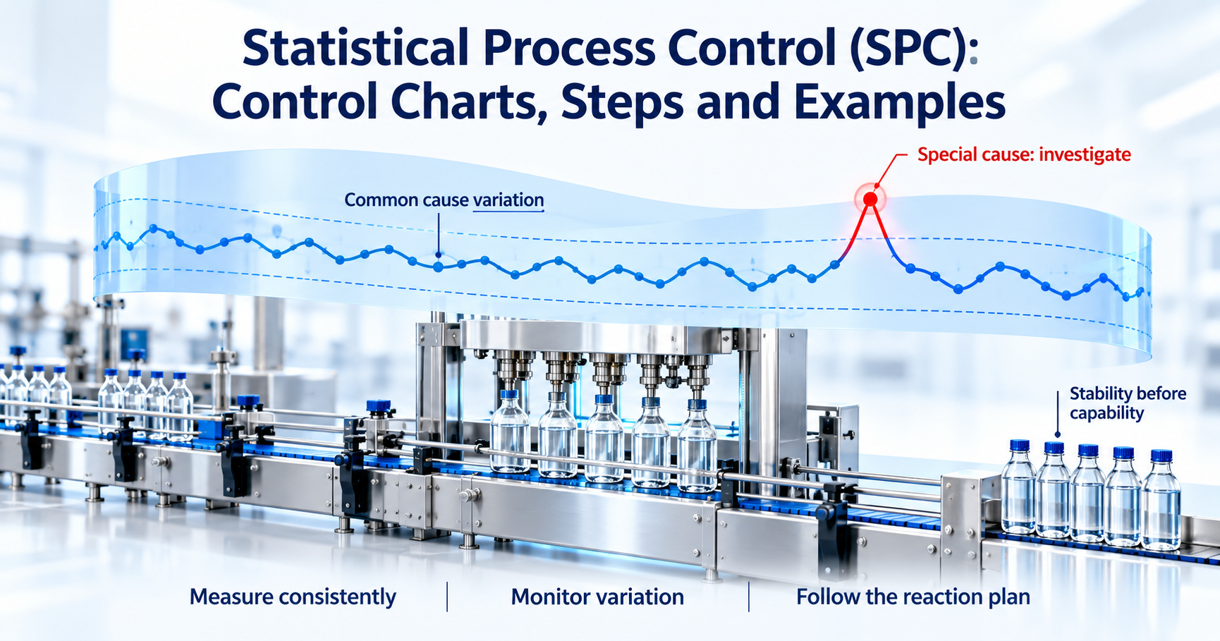
Statistical process control (SPC) is a method of monitoring a process with statistics so you can tell normal variation apart from real problems. Teams plot process data on control charts, compare each point with control limits calculated from the process itself, and act only when the chart signals a special cause. Used well, SPC catches problems early, cuts scrap and rework, and keeps a process stable enough to deliver consistent quality.
Key Highlights of Statistical Process Control (SPC)
- Statistical process control uses data, not guesswork, to decide when a process needs adjusting and when it should be left alone.
- The control chart is the core SPC tool. Walter Shewhart created it at Bell Telephone Laboratories in 1924.
- Variable data uses X-bar and R charts or individuals charts. Attribute data uses p, np, c and u charts.
- Control limits come from the process. Specification limits come from the customer. They answer different questions.
- Western Electric rules help you spot unusual patterns before a point falls outside the limits.
- A process must be stable before its capability indices, such as Cp and Cpk, mean anything.
- In Six Sigma, SPC is the main monitoring method in the DMAIC Control phase.
Introduction
Every process varies. Two bottles from the same filling line never hold exactly the same volume. Two calls to the same help desk never take exactly the same time. The real question is not whether variation exists, but whether the variation you see is normal for the process or a sign that something has changed.
That is the question statistical process control answers. Instead of waiting for a defect to reach a customer, or reacting to every small wobble in the numbers, SPC gives you a simple rule: watch the process with data, and step in only when the data says something unusual has happened.
SPC sits at the heart of modern quality control and project quality management. It is also one of the most practical skills in Six Sigma. If you are new to the methodology, it helps to first understand what is Six Sigma, because SPC is how Six Sigma teams protect the gains they make.
In this guide, you will learn the meaning of statistical process control, where it came from, the main types of statistical process control charts, how to read them, how to set up an SPC program step by step, which tools and software help, and how SPC connects to process capability and the DMAIC Control phase. A worked example ties it all together.
What Is Statistical Process Control?
The meaning of statistical process control is simple: it is a way to monitor and control a process using statistical methods, so the process keeps producing output that meets its target with as little waste as possible. ASQ: statistical process control describes it as applying statistical techniques to control a process, and that is a good working definition.
At the centre of SPC is one idea: variation comes from two kinds of causes.
- Common cause variation is the natural, built-in noise of a process. It comes from many small factors acting together, such as slight differences in raw material, room temperature, or operator technique. No single cause stands out, and the pattern is predictable over time. You reduce it only by changing the process itself.
- Special cause variation comes from a specific, identifiable event that is not part of the normal process. A worn tool, a new supplier batch, a sensor fault, or an untrained operator are typical examples. Special causes make the process unpredictable, and they can usually be found and removed.
A process showing only common cause variation is called stable, or in statistical control. Its output is predictable within a range. A process with special causes is unstable, and you cannot reliably predict what it will do next.
This distinction matters because the right response is different for each. If you treat common cause noise as a problem and adjust the process every time a reading moves, you add variation instead of removing it. W. Edwards Deming called this tampering. If you ignore a special cause, defects pile up. Statistical process control methods give you an objective way to tell the two apart.
History: Walter Shewhart
SPC began with Walter Shewhart, a physicist working at Bell Telephone Laboratories in the 1920s. Western Electric, which built telephone equipment for the Bell System, wanted parts that behaved consistently, but frequent adjustments on the factory floor were making results worse, not better.
In a short memo dated May 1924, Shewhart sketched the first control chart. He showed that you could set limits from the process data itself and use them to decide when to act. He later laid out the full theory in his 1931 book, Economic Control of Quality of Manufactured Product.
W. Edwards Deming, who worked with Shewhart, carried these ideas further. SPC was widely used in American wartime production during the 1940s, and after the war Deming taught it to Japanese engineers and managers, where it became part of the quality movement that reshaped Japanese manufacturing. In 1956, Western Electric published its Statistical Quality Control Handbook, which introduced the decision rules now known as the Western Electric rules. For a broader timeline, see Statistical process control on Wikipedia.
Today, SPC statistical process control is used far beyond factories, in hospitals, banks, software teams, call centres and logistics.
SPC vs Quality Inspection
Traditional quality inspection checks finished products against specifications and separates good units from bad ones. It is useful, but it has clear limits. It finds defects after they are made, it costs time and labour, and 100% inspection still lets some defects slip through because people get tired and miss things.
SPC works differently. It watches the process while it runs and flags a change before it produces a large number of defects. Think of inspection as sorting the output and SPC as steering the process.
| Aspect | Quality inspection | Statistical process control |
| Focus | The finished product | The process producing it |
| Timing | After production | During production |
| Approach | Detect and sort defects | Prevent defects by spotting change early |
| Data use | Pass or fail against specification | Trends and patterns against control limits |
| Cost of poor quality | Higher scrap and rework | Lower, because problems are caught sooner |
This shift from detection to prevention mirrors the wider move from quality control toward quality assurance and management. If you want to see how those ideas connect, read our guide on quality assurance vs quality management. In practice, most organisations still keep some inspection, but SPC reduces how much they need.
Statistical Process Control Charts
A control chart, also called an SPC chart or Shewhart chart, is a time-ordered plot of process data with three reference lines:
- Centre line (CL): the process average.
- Upper control limit (UCL): usually the centre line plus three standard deviations.
- Lower control limit (LCL): usually the centre line minus three standard deviations.
Why three standard deviations? Shewhart chose them as an economic balance. If a stable process is roughly normal, about 99.7% of points fall inside three-sigma limits, so false alarms are rare, but real shifts still show up quickly. For a refresher on how project teams use control charts, see our dedicated guide.
Statistical process control charts fall into two families, based on the type of data you collect:
- Variables data is measured on a continuous scale, such as weight, length, time, or temperature.
- Attributes data is counted, such as the number of defective units or the number of defects on a unit.
Variables charts usually come in pairs: one chart tracks the process centre, and the other tracks the spread. Attribute charts track a single statistic.
X-bar and R Charts
The X-bar and R chart is the classic pair for variable data collected in small subgroups, typically two to nine units, with four or five being most common.
- The x bar chart plots the average of each subgroup. It shows whether the process centre is shifting.
- The r chart plots the range (largest minus smallest value) of each subgroup. It shows whether the spread within subgroups is changing.
Control limits use the grand average and the average range, along with constants that depend on the subgroup size. For a subgroup of five, the X-bar limits are the grand average plus or minus 0.577 times the average range, and the R chart's upper limit is 2.114 times the average range, with a lower limit of zero.
Always read the R chart first. If the spread is out of control, the X-bar limits are not reliable, because they are calculated from the average range. When subgroups have ten or more units, teams usually switch to an X-bar and S chart, which uses the standard deviation instead of the range.
Individuals and Moving Range Charts
Sometimes you get only one measurement at a time. Examples include a daily chemical batch, monthly invoice processing time, or a slow, expensive test. Here you use the individuals chart with a moving range chart, often called the I-MR chart.
- The individual chart plots each single value.
- The moving range chart plots the absolute difference between each value and the one before it.
The average moving range estimates short-term variation. The individual limits are the average plus or minus 2.66 times the average moving range, and the moving range chart's upper limit is 3.267 times the average moving range. I-MR charts are popular in service and transactional processes, but they are more sensitive to non-normal data than subgroup charts, so check the shape of your data first.
p and np Charts
The p and np charts are for defectives, meaning units that either pass or fail.
- A p chart plots the proportion defective in each sample, for example the share of loan applications with errors each day. It handles sample sizes that change from one period to the next, although the control limits widen or narrow as sample size changes.
- An np chart plots the number of defective units. It needs a constant sample size, for example 200 parts checked every shift.
Both are based on the binomial distribution, so each unit must be classified as simply defective or not.
c and u Charts
The c and u charts are for defects, where a single unit can have several problems. A painted car door with three scratches is one defective unit but three defects.
- A c chart plots the count of defects per inspection unit when the area of opportunity stays the same, for example the number of flaws on each 10-metre roll of fabric.
- A u chart plots defects per unit when the area of opportunity changes, for example coding errors per 1,000 lines of code when each release has a different size.
Both rely on the Poisson distribution, which assumes defects occur independently of one another.
Chart Selection Table
Use this table to pick the right chart for your data.
| Data type | What you measure or count | Subgroup/ sample size | Chart to use | Example |
| Variables | Individual measurements | 1 | Individuals and Moving Range (I-MR) | Daily batch yield, monthly cycle time |
| Variables | Measurements in subgroups | 2 to 9 (constant) | X-bar and R | Fill volume of 5 bottles every 30 minutes |
| Variables | Measurements in subgroups | 10 or more | X-bar and S | Diameter of 12 shafts per hour |
| Attributes | Defective units (proportion) | Can vary | p chart | Percentage of invoices with errors each week |
| Attributes | Defective units (count) | Constant | np chart | Rejected parts in a fixed sample of 200 |
| Attributes | Defects per unit | Constant area of opportunity | c chart | Flaws per roll of fabric |
| Attributes | Defects per unit | Varying area of opportunity | u chart | Errors per 1,000 lines of code |
Reading a Control Chart
Reading a control chart comes down to one question: does this pattern look like random noise, or does it point to a special cause? A stable chart has points scattered around the centre line, most of them close to it, a few nearer the limits, and none outside them, with no obvious trends or cycles.
When you see a signal, the response is to investigate, not to adjust blindly. Find what changed, fix it if it is harmful, and keep it if it is an improvement you want to lock in. ASQ: control chart offers a useful checklist for this kind of review.
Control Limits vs Specification Limits
This is one of the most common points of confusion in SPC.
- Control limits are calculated from process data. They describe what the process is actually doing. They are the voice of the process.
- Specification limits are set by the customer, a design engineer, or a regulation. They describe what the output should be. They are the voice of the customer.
The two sets of limits answer different questions. Control limits tell you whether the process is stable. Specification limits tell you whether each unit is acceptable. A process can be in control and still make out-of-spec parts if its natural spread is too wide. It can also be out of control while every part is still within specification, which is a warning to act before defects appear.
For that reason, never draw specification limits on an X-bar chart. Averages vary less than individual values, so comparing averages with specifications for individual units gives a false sense of safety.
Western Electric Rules
A point outside the control limits is the most obvious signal, but it is not the only one. The Western Electric rules divide the area between the centre line and each control limit into three zones of one standard deviation each. Zone C is nearest the centre, Zone B is in the middle, and Zone A is next to the limit.
The four standard rules flag a likely special cause when:
- One point falls beyond the three-sigma control limit.
- Two out of three consecutive points fall in Zone A or beyond, on the same side of the centre line.
- Four out of five consecutive points fall in Zone B or beyond, on the same side of the centre line.
- Eight consecutive points fall on the same side of the centre line.
Rules 2 to 4 pick up smaller, sustained shifts that a single limit would miss for a long time. Other rule sets, such as the Nelson rules, add patterns like six points steadily rising or falling.
Use these rules with care. Each extra rule catches more real shifts, but it also raises the chance of a false alarm. Many teams start with Rule 1 and Rule 4, then add others where early detection matters. The NIST e-Handbook: process monitoring and control explains the statistics behind these trade-offs in more depth.
How to Implement SPC Step by Step
A statistical process control program does not need to start big. Most successful programs begin with one or two important processes, prove the value, and then expand. The three stages below cover the core work.
Select Critical Characteristics
You cannot chart everything, and you should not try. Focus on the characteristics that matter most to the customer, to safety, or to cost.
- Start with customer requirements, complaint data, and failure history to find the outputs that matter most.
- Look upstream for the process inputs that drive those outputs, such as oven temperature, line speed, or approval time. Charting a key input often warns you earlier than charting the output.
- Confirm your measurement system before you trust the data. A measurement system analysis, such as a gauge R&R study, tells you how much of the variation you see comes from the gauge or the person measuring rather than the process. If measurement error is large, your control chart will mostly show noise.
Collect Rational Subgroups
Rational subgrouping is the most important design choice in SPC, and the one most often done poorly. A rational subgroup is a small set of units made under nearly identical conditions, usually consecutive units taken close together in time.
The logic is straightforward. Variation within a subgroup should represent only common causes. Variation between subgroups can then reveal special causes that appear over time. If you mix units from two machines or two shifts into one subgroup, you hide the very differences you want to find.
Practical guidance:
- Take four or five consecutive units for each subgroup when using X-bar and R charts.
- Set a sampling frequency that matches how quickly the process can change. A fast, high-volume line may need a subgroup every 30 minutes, while a slow process may need one per day.
- Collect at least 20 to 25 subgroups before calculating trial control limits.
- Record the context alongside the data, such as the operator, material lot, and any adjustments. These notes make investigations much faster.
Set Control Limits and React
Once you have enough data, calculate trial control limits and plot the points.
- Check for special causes in the baseline: If points fall outside the limits and you can find and fix the cause, remove those points and recalculate. Do not remove points just because they look inconvenient.
- Freeze the limits: Once the process is stable, keep those limits fixed and use them to judge new data. Recalculating every day hides gradual drift.
- Write a reaction plan: For each type of signal, state who responds, what they check first, and when to stop the line or escalate. A chart without a reaction plan is just a picture.
- Review and recalculate only for a reason: Update limits after a deliberate, confirmed process change, not on a fixed calendar.
This discipline turns process monitoring from a reporting exercise into a real decision tool. Operators know exactly when to act, and just as importantly, when to leave the process alone.
Statistical Process Control Tools and Software
Control charts are the main statistical process control tools, but they work best alongside other basic quality tools. Histograms show the shape of your data, Pareto charts rank the biggest problems, check sheets make data collection consistent, and cause-and-effect diagrams help teams find the root cause once a chart signals a problem. Many of these appear in our list of Six Sigma Green Belt tools.
For the charts themselves, you have three broad options:
- Spreadsheets: Excel or Google Sheets work for learning and small pilots, and add-ins such as SigmaXL or QI Macros make charting easier.
- Statistical packages: Minitab and JMP are widely used by Six Sigma practitioners for analysis, capability studies, and charting.
- Real-time SPC systems: Dedicated statistical process control software, such as InfinityQS ProFicient, collects data directly from gauges and machines and alerts teams on the shop floor.
SPC Software Features
When comparing SPC statistical process control software, look for these features:
- Automatic data capture from gauges, sensors, and production systems, to cut manual entry errors.
- Support for all common chart types, including I-MR, X-bar and R, X-bar and S, p, np, c and u charts.
- Configurable rule checks, including the Western Electric rules, with real-time alerts.
- Built-in capability analysis that reports Cp, Cpk, Pp and Ppk.
- Fields for recording causes and corrective actions against each signal.
- Dashboards that show many lines or sites at once, plus audit trails for regulated industries.
The best tool is the one your team will actually use every day. A simple chart that operators check and act on beats an advanced system nobody looks at.
SPC Example
To see how the pieces fit together, consider a typical manufacturing case.
Filling Line Example
A beverage plant fills 500 ml bottles. The specification is 495 to 510 ml. The quality team takes five consecutive bottles every 30 minutes and measures fill volume, so an X-bar and R chart is the right choice.
After collecting 25 subgroups, they find a grand average of 502.0 ml and an average range of 3.5 ml. Using the constants for a subgroup of five:
- X-bar chart: UCL = 502.0 + (0.577 x 3.5) = 504.0 ml; LCL = 502.0 - 2.0 = 500.0 ml
- R chart: UCL = 2.114 x 3.5 = 7.4 ml; LCL = 0
The baseline shows no signals, so the team freezes these limits.
A few weeks later, the X-bar chart shows eight subgroup averages in a row above the centre line, between 502.4 and 503.6 ml. That breaks Western Electric Rule 4, even though no point is outside the limits. Shortly after, one average reaches 504.6 ml, above the UCL.
The operator follows the reaction plan, checks the filler, and finds that a pressure regulator drifted after routine maintenance. Once it is reset, the averages return to the centre line. Because the team acted on the run of eight points, they caught the drift early, and no bottle went outside specification. Overfill costs money too, so the early warning also cuts product giveaway.
SPC and Process Capability
Statistical process control tells you whether a process is stable. Process capability tells you whether that stable process can meet its specifications. You need both, and the order matters.
From Stability to Capability
Capability indices compare the natural spread of a process with the width of its specification. The two most common are:
- Cp = (USL - LSL) / 6σ. It measures potential capability, assuming the process is perfectly centred.
- Cpk = the smaller of (USL - mean) / 3σ and (mean - LSL) / 3σ. It measures actual capability, because it accounts for how far the process means sits from the centre of the specification.
Here, σ is the short-term, within-subgroup standard deviation, often estimated from a control chart as the average range divided by a constant called d2. Pp and Ppk use the overall standard deviation instead and reflect long-term performance.
In the filling line example, σ = 3.5 / 2.326 = 1.50 ml. That gives Cp = 15 / 9.0 = 1.66 and Cpk = (502.0 - 495) / 4.5 = 1.55. Many organisations treat a Cpk of 1.33 as the minimum for an existing process and 1.67 for critical or new processes, so this line is capable.
The key rule is stability first. If a process has special causes, its mean and spread keep changing, so any Cpk you calculate describes only a moment, not the process. Always confirm that the control chart is stable before you report capability. The NIST e-Handbook: process capability covers the formulas and assumptions, including what to do with non-normal data. Cpk sits alongside other Six Sigma metrics such as DPMO and sigma level.
SPC in the DMAIC Control Phase
The DMAIC process runs through Define, Measure, Analyze, Improve, and Control. By the time a project reaches the Six Sigma Control phase, the team has found root causes and made improvements. The job now is to make sure those gains last after the team moves on.
SPC is the main way to do that. In the Control phase, teams typically:
- Place control charts on the critical outputs and the key inputs identified during Analyze.
- Recalculate control limits using data from the improved process, so the charts reflect the new baseline.
- Confirm improved capability with a fresh Cpk study.
- Document charts, sampling plans, and reaction steps in a control plan in Six Sigma.
- Hand ownership of the charts to the process owner, with training on how to read and respond to them.
Without this step, many processes slowly drift back to old habits. SPC gives the process owner an early warning long before results slip far enough for a customer to notice.
Conclusion
Statistical process control gives teams a clear, data-based way to understand their processes. Control charts separate common cause variation from special cause variation, so you fix real problems and leave normal noise alone. Pair the right chart with sound subgrouping, fixed control limits, clear rules, and a reaction plan, and SPC becomes part of daily work. Combine it with capability analysis and the DMAIC Control phase, and it protects every improvement you make.
If you want to apply these methods to real projects, the Lean Six Sigma Green Belt certification covers SPC, capability analysis, and the full DMAIC toolkit in depth. You can also check your readiness with a Lean Six Sigma Green Belt practice test.








 Lowest-Price Challenge













 Personalized Path



.webp)


 USA
 Canada
 India
 UK
 Australia
 Singapore


